Last time a power balance showed that theory and tests were in the same car park.

This time we’ll see if motor torque and tractive effort make sense.

Here is the graph of torque and power vs motor speed that we developed in post 3.

How can we get a graph of tractive effort vs vehicle speed? 

We will start at the wheel/road contact and work our way to the motor.

The torque transmitted from the drive shaft to the wheel is

TW = TE*(d/2)             TE is Tractive effort and d/2 is the wheel radius

TW is the output torque from the transmission system.

If we neglect losses for the moment, the input torque to the transmission is:

 TM = TW*GR              GR is the gear ratio

If we now include the transmission losses, this input torque becomes

 TM = TW*GR/eta         eta is the transmission efficiency

And, of course, TM is the output torque of the motor.

A bit of algebraic fiddling gives:

TE = TM*GR/(d/2)*eta

The road speed, v is:

v = (n*2*pi/60)/GR)*(d/2)

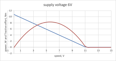
These two calculations give us this graph for TE vs V (in this case for a supply voltage 6V)

Here are curves of tractive effort vs car speed for various supply voltages, plotted on the same graph as total drag.

Now we are getting there. The balancing speed for any supply voltage is the speed where the curves of tractive effort and total drag cross. In this case, for 6V it’s about 17.5km/h, and for 7.2v it’s about 21km/h.

Our results in test 2 were 22km/h. It looks good, but is the transmission efficiency of the grasshopper really as low as the 0.6 (60%) that I put in my model. And what about the rolling coefficient (0.08) and the aerodynamic drag coefficient (0.07).

We’ll come back to this. But next we’ll look at the battery.