
To find the speed of the car we balance the tractive effort at the drive wheels against resistance to motion (drag)..
We will calculate the drag components described last time:
- rolling resistance,
- aerodynamic resistance and
- gravity (hill climbing).
Rolling resistance
We saw last time that we can express rolling resistance as a fraction of the weight.
The mass of our Grasshopper is given as 1,18 kg, so the weight is 1.18*9.8 N or 11.6 N.
Selecting a coefficient of rolling resistance is tricky. If it were a regulation passenger car we could use some general number, such as 0.015, with some confidence, but the situation is less clear with a model. The nature of the road matters – is it smooth bitumen or rough gravel for example. And a 1/10 scale model might be different from full-size car.
To get some idea of rolling resistance for small vehicles, I measured it on land yachts I made earlier.

vehicle A: wheel diameter about 25mm, wheels cut with scissors from 5mm foam board

vehicle B: wheel diameter about 54mm, wheels made from the top of a soft drink can
I found the rolling resistance of each vehicle on three different surfaces by finding the gradient to keep them rolling.

wheel on ribbed table mat 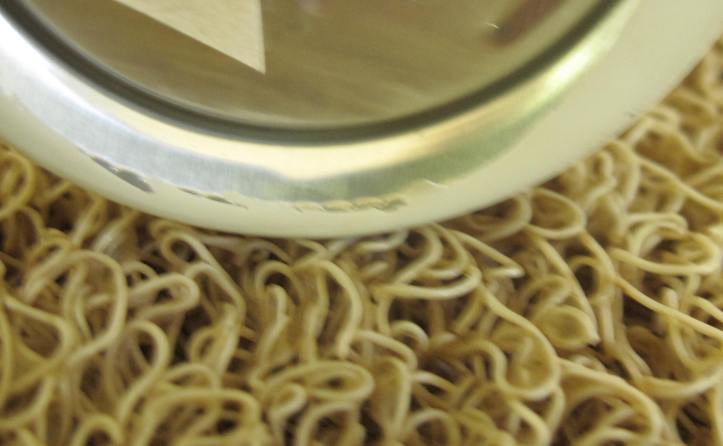
wheel on door mat 
vehicles on door mat 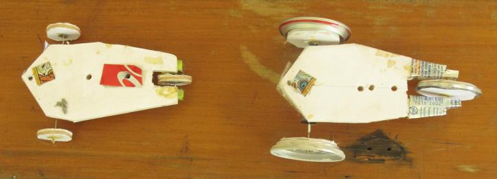
vehicles on wooden plank 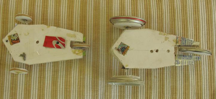
vehicles on table mat
| surface | vehicle | gradient for keeping rolling |
| hard timber | A | 0.022 |
| hard timber | B | 0.011 |
| ribbed table mat | A | 0.045 |
| ribbed table mat | B | 0.032 |
| open structure door mat | A | 0.060 |
| open structure door mat | B | 0.052 |
Measurements with the Grasshopper would be good, but for the moment we’ll assume CR = 0.04.
That gives a rolling drag of 1.18*9.8*0.04, or 0.463 N.
Aerodynamic drag
The challenge with this calculation is finding an appropriate drag coefficient, CD.
As with the rolling coefficient, this will depend on the scale factor. One particular factor that is often used to take account of this is Reynolds’ number:
RE = rho*v*d/mu where rho and v are as before and mu is dynamic viscosity of
the fluid (air in this case, for which mu = 18 Ns/m^2 x10^-6)
For the moment we’ll assume CD = 0.5.
Gravity drag
This is the easiest mathematically, but we seldom have an accurate value for the gradient.
Gravity Drag = m*g*sine(gradient)
in our case:
Gravity Drag = 1.18*9.8*sine(gradient) for most gradients, sine(gradient) is
near enough to the gradient as a ratio
(eg 1:10 would be 0.1)
A first look at balance.
For steady speed, the power required at the contact of the wheel with the road must be available from the motor.
Power required at the road is:
PD = (total drag)*(speed) drag in N, speed in m/s, power in W
Power from the motor is:
PM = (torque)*(rotational speed) W torque in Nm, rotational speed in radian/s
(1 revolution = 2*pi radians), power in W
There will be losses in the transmission, so the power from the motor that reaches the road is:
PR = eta*PM where eta is transmission efficiency
Transmission efficiency is something to explore with tests on the Grasshopper, but for now I will take 70%.
The table shows the calculated drag power and the maximum available power from the motor (after transmission losses) at a supply voltage of 6V.
| speed, km/h | drag power, W | motor power after losses, W |
| 10 | 2.11 | 24.5 |
| 20 | 4.12 | 24.5 |
| 30 | 9.08 | 24.5 |
| 40 | 17.53 | 24.5 |
| 50 | 30.62 | 24.5 |
At first glance it might look as though the Grasshopper could reach 40km/h, but this calculation assumes that maximum power is available at each speed, which is not the case. Top speed in our tests was about 17km/h.
We have to match the motor speed to the car speed. That’s all about gearing. We will look at that next.
